Creating Neural Network from Scratch in Python
Table of Contents
In my previous post, I had introduced neural networks at a very high level. If you haven’t read that post then I suggest reading it first before continuing. It will give you an idea of what we are going to accomplish today.
In this post, I am going to show you how to create your own neural network from scratch in Python using just Numpy.
For this tutorial, we are going to train a network to compute an XOR gate ($$X_1, X_2$$). This example is simple enough to show the components required for training.
| $$X_1$$ | $$X_2$$ | $$X_3$$ | $$Y$$ |
| 0 | 1 | 1 | 1 |
| 1 | 0 | 1 | 1 |
| 1 | 1 | 1 | 0 |
| 0 | 0 | 1 | 0 |
Here is how the network is going to look:
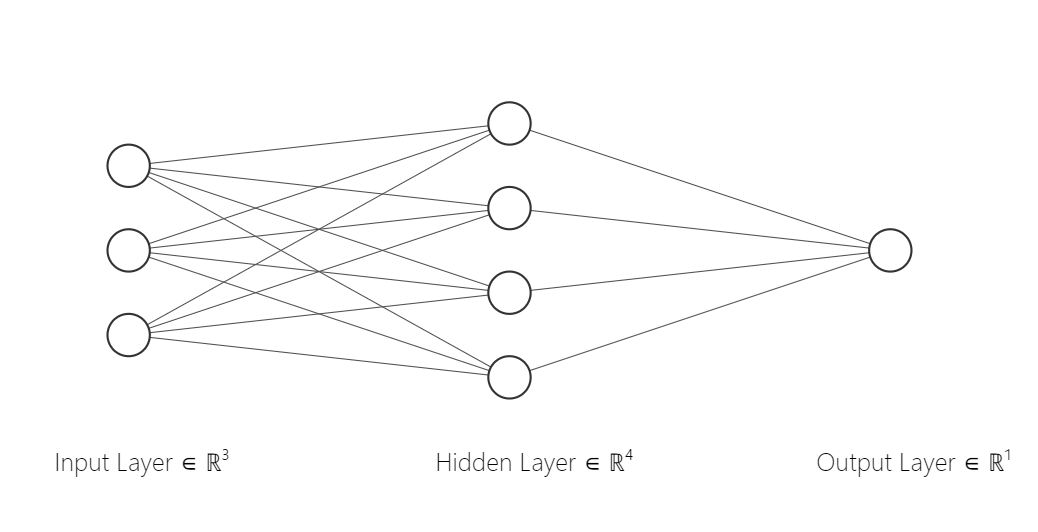
Data
The first layer is the input layer, the second is the hidden layer and the last layer is the output layer.
Let’s start coding by initializing the training data.
import numpy as np

def sigmoid(x):
    return 1.0/(1.0 + np.exp(-x))

def sigmoid_prime(x):
    return sigmoid(x)*(1-sigmoid(x))

#Create dataset
X = np.array([[0,1, 1], [1,0, 1], [1, 1, 1], [0,0,1]])
Y = np.array([ [1], [1], [0], [0]])
I have also defined the sigmoid function and its derivative function as we will need it later.
Creating the network
np.random.seed(1) # good practice
hidden_weights = np.random.randn(3,4)
output_weights = np.random.randn(4,1)

hidden_bias = np.random.randn(4)
output_bias = np.random.randn(1)
Since the first layer is the input layer, we essentially deal with two sets of weights. The first set is from the 3 input units to the 4 hidden units. The second set maps the hidden units to the output unit.
I have also included bias for completeness. While this simple example works just fine without biases, including them in the calculation keeps our network consistent with the one shown in the previous post.
The randn function assigns weights from a uniform normal distribution. There are cleverer ways to initialize weights but this is good enough for the current example.
Finally, remember to seed the random function. This will initialize the weights similarly in each run. You don’t want the initialization to change between executions. It becomes crucial when optimizing the hyperparameters. Random weights initialization will lead you to believe that the improvement was because of a particular selection of hyperparameter leaving you with a sub-par model.
Forward Pass
If you remember from the previous post the output of the network is $$\hat{y} = \sigma(x*w + b)$$, w represents the weights and x represents the output from the previous layer.
The code for the forward pass is very simple.
hidden_activation = sigmoid(np.dot(X, hidden_weights) + hidden_bias)
output_activation = sigmoid(np.dot(hidden_activation, output_weights) + output_bias)
Backward Pass
This is where things get interesting. Up till now, we have just created a simple neural network which takes in data and makes a prediction. Initially, the network does not predict the right value of Y given the input. To be able to train a network we need a loss function. Loss function tells by how much the network deviates from the actual input.
We are going to use the Mean Squared Error Loss function defined as
$$\frac{1}{n}\sum_{i=1}^{n}(y_i - \hat{y}_i)^2$$
Here n is the total number of training examples. $$\hat{y}_i$$ represents the actual label for the training example.
Our motive is to adjust the weights so that the predicted output is closer to the required output. That is, the loss is reduced. Let’s just focus on a single training example.
$$J = (y - \hat{y})^2$$
This can be written as
$$J = (\sigma(x*w + b) - y)^2$$
This is the activation from the last layer. We want to see how much effect does the weights of the last layer have on the loss. Recall that the derivative at a point in a graph represents its slope.

The above image represents a curve with its derivative at the point in red. The loss function can be considered as the above curve but in multiple dimension (it actually forms a hyperplane). Trying to reduce the loss is similar towards moving in the valley in the above curve.
We can continue calculating the slope (derivative) and taking a step towards the valley. This is essentially what backpropagation does. Let’s take a partial derivative of the loss function (we are ignoring the bias for now)
$$\frac{\partial J}{\partial w} = 2*(\sigma'(x*w + b)*x)$$
Further, taking derivative with respect to bias
$$\frac{\partial J}{\partial b} = 2*(\sigma'(x*w + b))$$
This shows how much effect the weights in the last layer have on the final cost. Similarly, we can write the cost function in terms of weights in the hidden layer.
$$J = (\sigma(\sigma(x*w_1 + b_1)*w_2 + b_2)- y)^2$$
Taking partial derivative with respect to $$w_1$$ will give the effect of $$w_1$$ on the loss function. To become comfortable with the calculation I suggest calculating the derivative of the above equation on your own.
$$\sigma'$$ is the derivative of $$(\sigma)$$. With calculation it can be shown that $$\sigma'(x) = \sigma*(1-\sigma(x))$$. This is what we have used in the function above.
After iterating over the entire training data and accumulating the change in weights, the neural network is updated as follows.
$$w = w - \frac{1}{n}\sum_{i=1}^n \frac{\partial J}{\partial w}$$
$$b = b - \frac{1}{n}\sum_{i=1}^n \frac{\partial J}{\partial b}$$
delta_output_weights = (output_activation - Y) * sigmoid_prime(output_activation)
delta_hidden_weights = delta_output_weights.dot(output_weights.T) * sigmoid_prime(hidden_activation)
output_weights -= hidden_activation.T.dot(delta_output_weights)
hidden_weights -= X.T.dot(delta_hidden_weights)
output_bias -= np.mean(delta_output_weights)
hidden_bias -= np.mean(delta_hidden_weights, axis=1)
Putting It All Together
Finally, the entire code looks like this
And you can see the result below
Loss:  0.5013730688788007
Loss:  0.4664830127093482
Loss:  0.24207358013744795
Loss:  0.09891100378926312
Loss:  0.087323152676015
Loss:  0.06892222408037366
Loss:  0.05528837086156295
Loss:  0.027425185939300573
Thanks for reading 😎